How to Size a Transformer for Factory Expansion

Quick Takeaway

• Size the expansion from time-aligned electrical demand: establish the existing load, convert each new load on the correct kW/kVA basis, and include defined future loads once.
• In the worked example, overlapping production needs 700 kVA; enforceable staggering reduces the governing maximum to 540 kVA against a 630 kVA nameplate.
• A result below nameplate only makes retention a candidate. Check site thermal capability, motor-start voltage dip, harmonics and phase loading, and the surrounding distribution system.

Start with the load the transformer will actually see

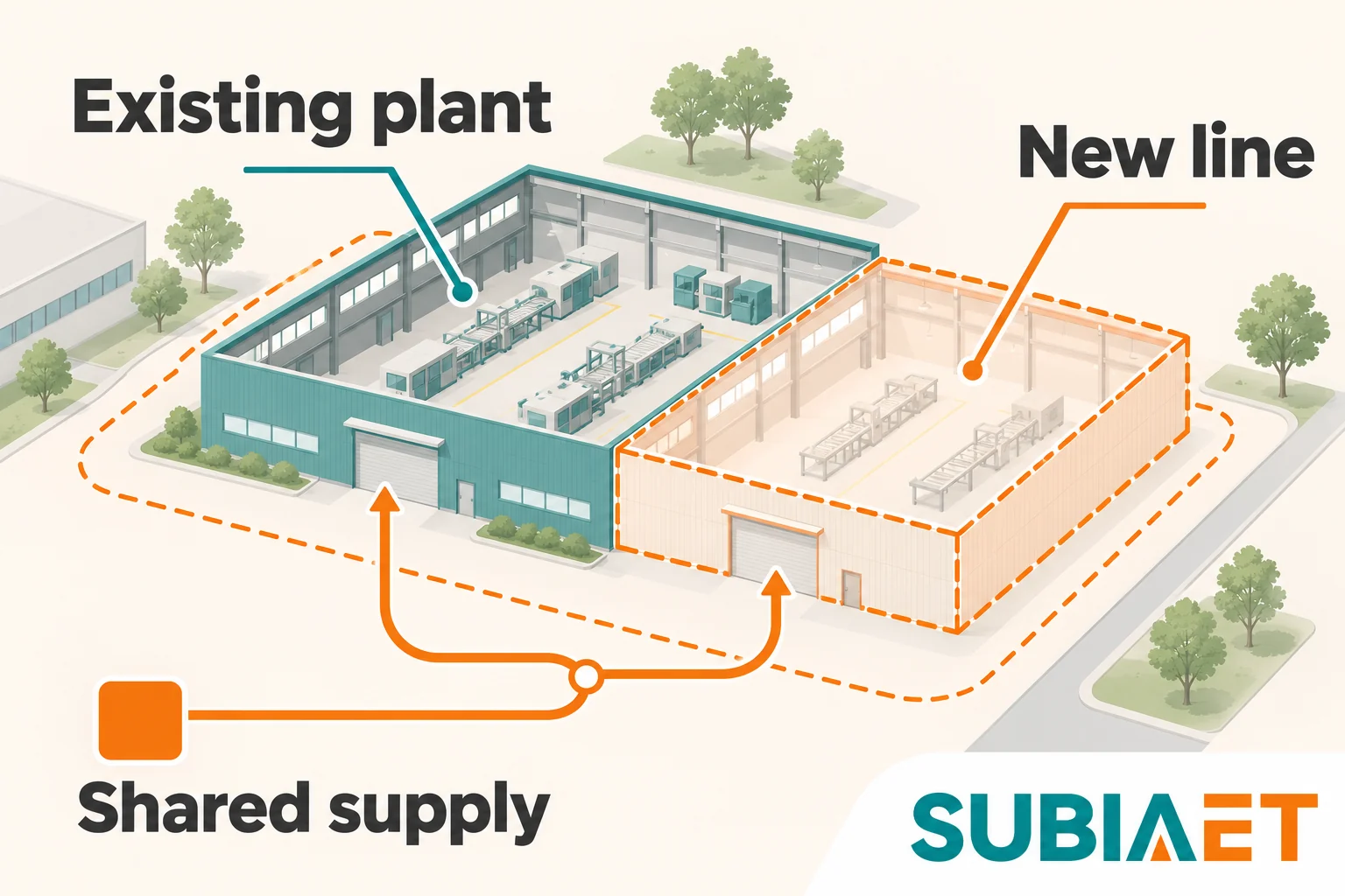
The central question in any factory expansion is whether the existing transformer can carry the new total demand, or whether something needs to change. The answer cannot come from adding up equipment nameplates or applying a universal margin. It requires comparing time-aligned load — the existing demand plus new operating demand plus any committed future load — against the capacity actually available under site conditions, all referred to the same supply boundary.

The supply boundary is the point where the transformer secondary feeds the factory distribution system: everything downstream of that point is the transformer’s load. The boundary matters because load records collected at the meter on that secondary are directly comparable to the transformer’s kVA rating, while readings taken further downstream, at individual distribution boards or sub-meters, need to be traced back to the common point before they can be summed.

A factory expansion can change more than the connected load list. It may change the production schedule, shift how much of the existing load runs simultaneously, and add committed future loads that belong in the sizing calculation even before they are energized. All of these changes need to be reflected in the demand calculation before any judgment about transformer adequacy is possible.

Build a usable baseline and load list

Before calculating anything, establish what the existing transformer is actually supplying and what records are available to support it.

Measuring the existing demand. Energy meters and power analyzers record demand as average power over a configured interval. The peak demand value from such a record represents the highest average over that interval within the reset period. That is not the same as an instantaneous peak, and it cannot directly tell you about short-duration events like motor starts or fault conditions. Confirm which parameter the meter records, the averaging interval, the peak timestamp, and whether the history has been reset. Schneider Electric’s power-demand explanation describes this averaging distinction.

For the transformer sizing baseline, the relevant quantity is apparent power in kVA at the supply boundary. If the existing meter records active power (kW) and power factor (PF), use paired readings from the same operating condition to calculate kVA = kW / PF; do not combine a maximum kW reading with an unrelated average PF. For interval records, confirm how the meter calculates and aggregates these quantities, and prefer its directly recorded kVA demand where available. If you have line voltage and line current, balanced three-phase kVA = √3 × V_LL × I_L / 1000. Do not mix these paths and apply PF twice.

Operating conditions vary. A factory with two-shift operation may have a substantially different peak in the morning production window compared with a maintenance-only window. Record the peak value for each significant operating mode — production peak, low-demand overnight window, seasonal peaks — and note which loads are present in each. This distinction matters directly when expansion changes which window carries the highest simultaneous demand.

Also record per-phase load distribution. Uneven loading may overheat the most heavily loaded phase or trigger protection before the total three-phase capacity appears exhausted, so a balanced-load assumption needs to be checked against reality.

Assembling the new load list. For each new load being added in the expansion, record:

• The power basis: electrical input kW, motor shaft kW (nameplate), or nameplate kVA
• Voltage and phase
• Operating duty and schedule (continuous, intermittent, which production window)
• Start method (direct-on-line, soft-starter, variable speed drive)
• Whether the load is nonlinear (drives, rectifiers, switch-mode power supplies)

For the worked example, assume the factory has the following operating readings and planned loads. The operating kW values are electrical input; the new-load utilization values are explicit assumptions for this example, not default industrial factors.

Keeping the future load on a separate row is deliberate. It is an already-approved load that belongs in the final capacity decision, but it should not be mixed into the existing baseline or treated as speculative margin.

Convert power without counting the same adjustment twice

Before summing loads, every item must be on the same electrical basis. The most common error is applying a correction that has already been embedded in the starting value.

Three distinct starting points exist:

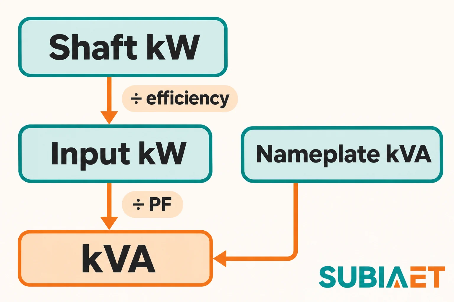
A motor nameplate states shaft power in kW — mechanical output at the coupling. To find the electrical input kW that the transformer must supply, divide by efficiency: input kW = shaft kW / η. Then, to get the apparent power the transformer sees, divide by power factor: input kVA = input kW / PF. Both steps are needed because the motor rating describes mechanical output, not electrical demand. This distinction is set out in Schneider Electric’s motor-power relationships.

If a load is already described in electrical input kW — a resistive heater, a process unit specified in consumed electrical power, or a motor table that states absorbed power rather than shaft power — apply only the PF step: kVA = input kW / PF. Do not divide by efficiency a second time: doing so would overstate electrical input power and therefore the calculated kVA.

If a nameplate states kVA directly, use it without further correction. The apparent power is already expressed.

Utilization and coincidence. These two concepts have specific meanings, and conflating them leads to either double-counting or missing a reduction.

Utilization describes how an individual load operates relative to its own nominal rating. A process line with a 90 kW nameplate that typically draws 72 kW under its normal operating cycle has a utilization of 0.80 (72/90). This is a property of that specific load and its duty cycle, derived from knowledge of how it operates — not from a generic table.

Coincidence describes what fraction of the individual maxima actually occur simultaneously at the group level. If all loads in a group genuinely run at the same time and at their utilization levels, the coincidence factor is 1.0: total group demand equals the sum of individual operating demands. If some loads are genuinely staggered, the coincidence factor is less than 1.0.

The important discipline is not to apply both a utilization factor and a coincidence factor unless you have clear evidence for each from the actual operating conditions. Applying a generic coincidence factor on top of an already-reduced utilization estimate can invent a second reduction. Schneider Electric’s demand-estimation guide distinguishes individual utilization from group coincidence; both need a defensible operating basis.

For loads with differing power factor angles, arithmetic addition of kVA values is not exactly correct — the vector sum of complex powers would be needed. In the balanced sinusoidal scenario below, every load has the same 0.90 lagging PF, so scalar kVA addition is consistent with that model. With only approximately equal PF angles, it becomes an approximation. Schneider Electric’s apparent-power explanation identifies this aggregation limitation. When the PF mix is wide — for example, a mix of motors at 0.80 lagging and resistive loads at unity — the aggregate PF needs to be determined from the actual load mix rather than assumed.

Calculate two operating schedules for the same expansion

Assume the existing transformer has a 630 kVA nameplate rating. The existing factory reaches its production peak at 432 electrical-input kW at 0.90 lagging PF, giving 480 kVA. In a later production window — after the main production shift — the existing load is 288 kW at the same PF, giving 320 kVA. These are the two distinct windows that become relevant when the expansion changes the schedule.

The expansion adds three new loads, all operating together in the new production window:

• Process line: 90 kW nameplate, 0.80 utilization = 72 kW operating
• Auxiliaries: 100 kW nameplate, 0.60 utilization = 60 kW operating
• Services: 30 kW nameplate, 1.00 utilization = 30 kW operating

Sum = 162 kW. All scenario loads are assumed balanced, sinusoidal, and operating at 0.90 lagging PF. With that common PF assumption, 162 kW / 0.90 = 180 kVA. No additional coincidence reduction is applied because the three loads are stated to operate together in the new window; a further reduction would require specific evidence of staggering among them.

A separately approved future load of 36 kW = 40 kVA also operates in the new production window. This is a defined committed load, not a speculative contingency.

Why utilization values are taken as given, not reduced further. The utilization factors (0.80 for the process line, 0.60 for auxiliaries) already reflect how those loads operate under their normal duty cycle. Applying a further simultaneous-use factor on top of these would require evidence that some of those loads do not run at the same time within the new production window — which is not stated in the scenario. The sum of 162 kW therefore represents the expected simultaneous demand from the new loads during their window, with the utilization already embedded.

Two cases arise depending on the production schedule.

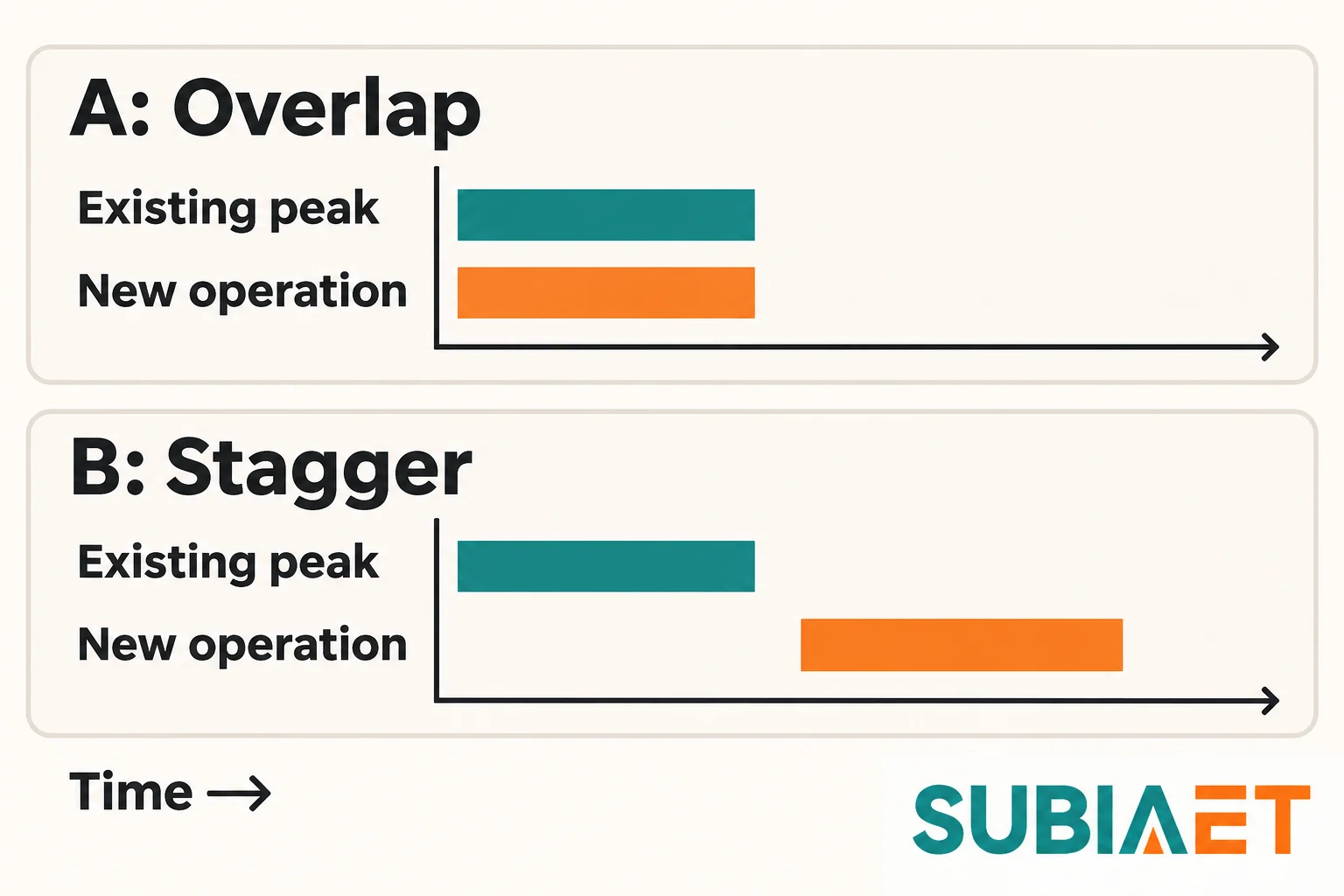
Case A: The new production window is scheduled to overlap with the existing morning peak. Both old and new loads run simultaneously:

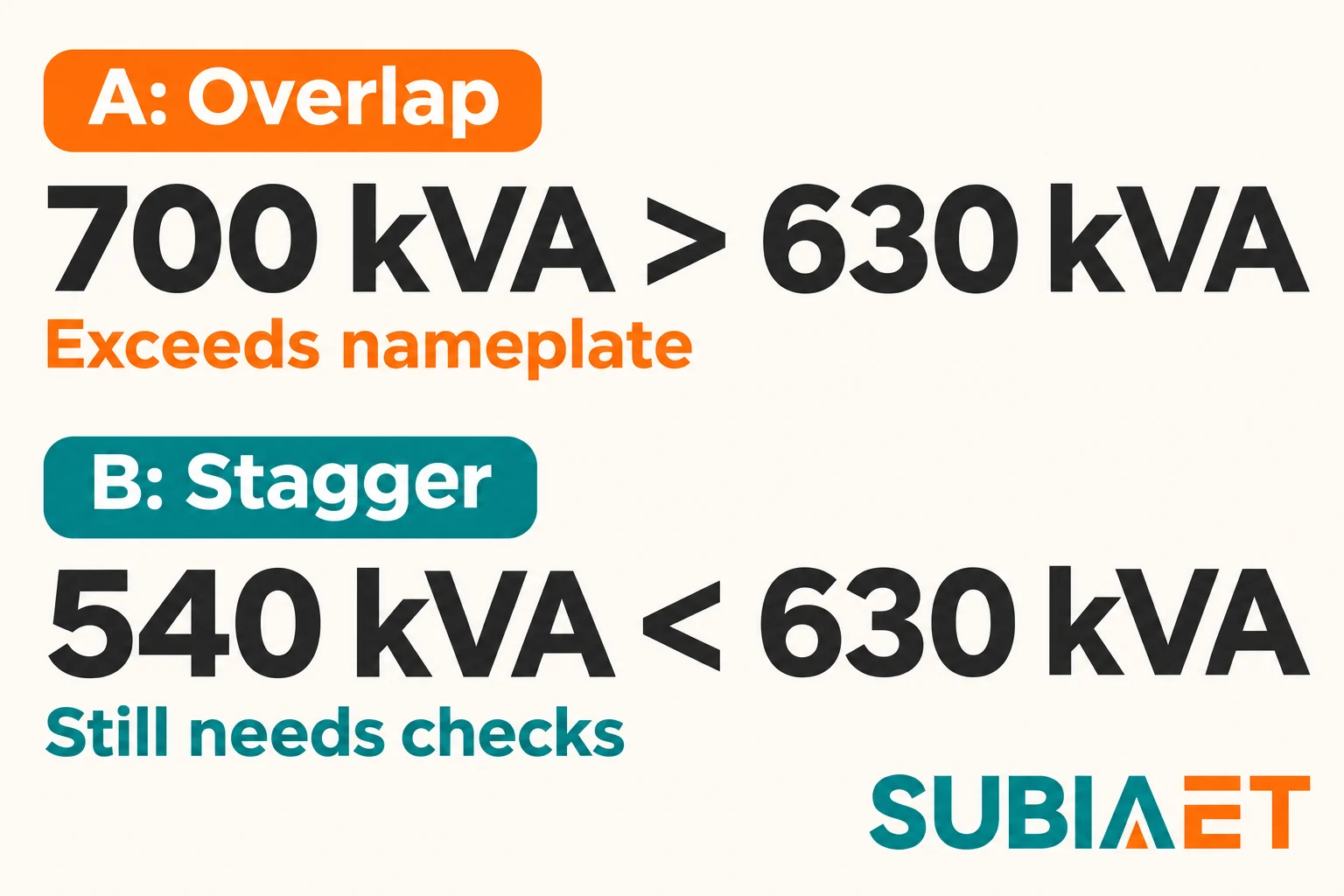
700 kVA exceeds the 630 kVA scenario nameplate. With this schedule, the expansion cannot proceed without either changing the operating plan or obtaining additional or replacement supply capacity.

Case B: The new production window and its future load are enforceably moved to the lower-demand window (288 kW / 320 kVA). The original peak of 480 kVA continues to exist in the morning shift, unchanged:

The governing maximum in Case B is 540 kVA — the higher of the new-window total (540) and the unchanged morning peak (480). 540 kVA is below the 630 kVA scenario nameplate.

What these numbers do and do not decide. The 630 kVA figure is the transformer’s scenario nameplate rating. It is not a confirmed available continuous capacity on the specific site, because continuous thermal capability depends on actual ambient temperature, installation cooling, and load history — none of which are established by the nameplate alone.

700 kVA in Case A means the expansion cannot proceed under that schedule at the existing transformer rating, regardless of other checks. Something must change: the schedule, the supply capacity, or both. This does not automatically imply an 800 kVA replacement; the appropriate next rating depends on the full load picture and site conditions, which an engineer and the transformer supplier need to assess together.

540 kVA in Case B means the transformer is a candidate for retention — but candidate status is conditional on the four parallel checks in the next section. A result below the nameplate does not confirm suitability. It means the schedule option is worth pursuing through those checks.

Before the future 36 kW load is installed, the totals would be 660 kVA (Case A) and 500 kVA (Case B). The comparison above uses the planned ultimate load throughout, as the future load is already committed.

Check the conditions that a kVA total cannot settle

A demand total in kVA is a necessary input, not a sufficient one. Four parallel checks must be completed before any conclusion about transformer suitability can be drawn.

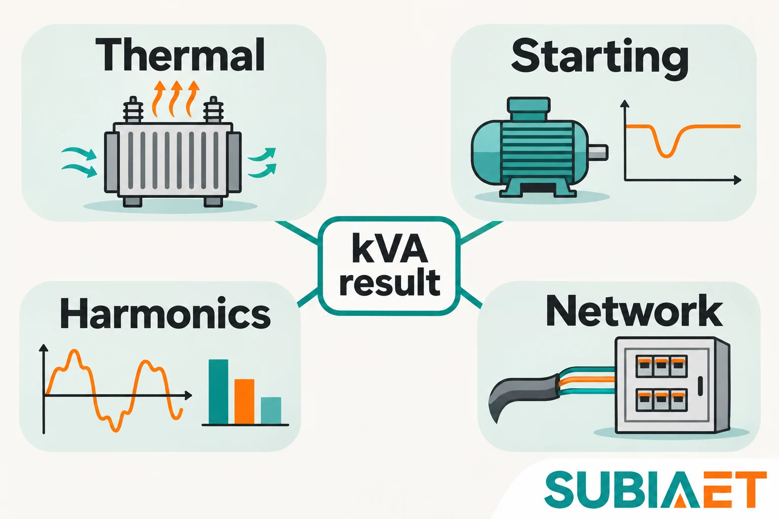
1. Continuous thermal capability and site cooling. A transformer’s nameplate rating is established under defined reference conditions — typically a specific ambient temperature and cooling arrangement. Ambient temperature above the unit’s rating conditions, restricted ventilation, or inadequate heat removal can reduce available continuous capacity or require changes to the installation. The existing transformer’s rated cooling method (ONAN, ONAF, or other) and the actual installation environment need to be confirmed. If the site operates at elevated ambient temperatures for extended periods, the effective available capacity may be meaningfully lower than 630 kVA. This check requires the transformer’s actual thermal characteristics and the site’s measured ambient conditions — not just a nameplate comparison.

2. Motor-start voltage dip. Starting current can exceed normal running current, depending on the motor, driven load and starting method. The transient current, interacting with the supply and transformer impedance, can depress the secondary-bus voltage. If that voltage dip exceeds what connected equipment can tolerate — motors may stall, sensitive controls may trip, lighting may flicker perceptibly — the starting event is a problem even if the steady-state running demand is well within the transformer’s rating.

Running kVA alone does not establish whether motor starting is acceptable. The relevant inputs are the motor’s starting current characteristic, the starting method and its actual current and torque characteristics (direct-on-line, soft-started or drive-controlled), whether multiple motors start simultaneously, the transformer’s percentage impedance, and the upstream network impedance. An averaged demand record from a metering system cannot reveal this event; it needs to be assessed separately using motor start data and transformer impedance.

3. Harmonics and phase imbalance. Variable-speed drives, rectifiers, and switch-mode power supplies draw non-sinusoidal current. Harmonic currents can increase winding eddy-current and other load-related losses beyond what a fundamental-frequency kVA figure indicates, causing additional heating. The thermal tolerance of a particular transformer to harmonic content depends on its design — a transformer with higher harmonic tolerance does not eliminate harmonics from the system; it only tolerates the additional heating better. If the expansion adds significant VSD-driven loads, assess the harmonic current and the transformer’s suitability for that duty. HPS explains why harmonic-current tolerance does not eliminate harmonics.

Phase imbalance adds a related concern. If single-phase loads are distributed unequally across phases, the most heavily loaded phase may overheat or its protection may operate before the total three-phase demand reaches the transformer’s rating. This is a practical risk in factories where lighting, small tools, and office loads are connected phase-to-neutral without careful balancing. The expansion is a good opportunity to review phase loading across the new and existing distribution.

4. Downstream cables, switchgear, protection, fault duty, and upstream supply. A transformer upgrade (or even retention at higher loading) has consequences that extend in both directions. Downstream, the cables, busbars, switchgear, and circuit breakers must be rated for the currents that the new loading will produce. Physical spare capacity in a distribution board — an empty slot — does not mean the board’s busbars, main breaker, or incoming cable can carry additional load. Each needs to be confirmed.

A larger transformer can increase prospective secondary fault current. The result depends on its actual percentage impedance, kVA rating, upstream source impedance and connecting conductors; a larger unit does not necessarily have a lower percentage impedance. Recalculate the fault level and check the relevant breaking and withstand ratings rather than assuming the old study remains valid.

Upstream, the utility supply connection and any medium-voltage switchgear have their own limits. The utility’s available fault level, its contracted demand, and any switchgear ratings need to be checked against the new loading scenario. These checks are outside the transformer kVA calculation itself but are part of the same project decision.

Turn the result into a transformer enquiry

The calculation above produces a structured set of inputs that can be used directly to frame an enquiry to a transformer supplier. A useful technical enquiry includes:

• The operating scenarios and load table (as shown above), with Case A and Case B clearly distinguished
• Primary voltage, secondary voltage, and system frequency
• Motor start data: largest motor kW, starting method, permitted voltage dip at the busbar
• Harmonic load content: estimated percentage of VSD or rectifier loading, any existing harmonic measurement
• Ambient temperature range, installation type (indoor substation, outdoor pad-mounted, ventilated enclosure), and site altitude
• Existing transformer details: nameplate kVA, impedance percentage, cooling method, age, and load history if available
• Committed future loads and their timescale
• Continuity of supply constraints: whether a changeover outage is acceptable, or whether parallel supply must be maintained during any transition

This information allows a supplier to confirm whether the existing unit is thermally suitable under site conditions, or to propose appropriate options if it is not.

For further background on transformer types relevant to industrial facilities, SUBIA’s transformer product range covers both oil-immersed and dry-type options. The industrial facilities application page addresses factory expansion scenarios including the types of data inputs useful for a transformer enquiry.

Frequently Asked Questions

Can I use nameplate totals to size a transformer for an expansion?

Use nameplates as inputs, not as the complete demand calculation. Some loads genuinely operate together at full input, so a reduction is not always justified. Other loads operate part-loaded or in separate windows. Motor shaft kW also needs conversion to electrical input and apparent power; adding uncorrected shaft-kW numbers can understate transformer demand. Establish the unit basis and operating schedule first, then apply only supported utilization and coincidence assumptions.

Is 25% spare capacity always needed after calculating the kVA total?

There is no universal 25% rule that applies across all factory expansions. The right margin, if any, depends on specific conditions: the likelihood of further load growth, whether the committed future load has already been included in the calculation, the thermal derating of the transformer at the actual site ambient, and project risk tolerance. In the scenario described here, the 36 kW future load is already included in the 540 kVA and 700 kVA totals — it is not a contingency reserve. Adding an arbitrary 25% on top of an already-conservative calculation that includes all defined future loads may displace a usable option unnecessarily. What matters is completing the four parallel checks (thermal, starting, harmonics, downstream/network) and ensuring that all defined loads are actually in the demand figure. A generic percentage margin is not a substitute for those checks.

Does a lower running kVA prove that motor starts will be acceptable?

No. Running kVA and motor-start voltage dip are fundamentally different phenomena and must be assessed separately. Starting current can substantially exceed running current, with magnitude and duration depending on the motor, driven load and starting method. This surge of current flowing through the transformer’s impedance depresses the secondary voltage. The severity depends on the motor’s starting current magnitude, the transformer’s percentage impedance, and the upstream network impedance — none of which are captured in a demand kVA figure. A transformer comfortably within its kVA rating during steady-state operation can still produce unacceptable voltage dips on starting a large motor, causing other connected loads to malfunction. To assess starting, you need the motor’s starting current characteristic (or its kVA at start), the starting method, any simultaneous-start scenarios, and the transformer’s impedance data. Schneider Electric’s motor-fed transformer FAQ explains why starting and voltage depression need separate consideration.

Does staggering the new production to a lower-demand window avoid replacing the transformer?

Staggered operation reduces the simultaneous demand and in this scenario brings the governing maximum from 700 kVA down to 540 kVA, which is below the 630 kVA scenario nameplate. That makes the existing transformer a candidate for retention. However, two conditions must hold for this to be a genuine solution rather than a nominal one. First, the schedule shift must be reliably maintained in every operating mode that relies on it — a verbal agreement to run new equipment in the off-peak window is not a load limitation in any technical sense; the plan needs suitable operational controls or load management, including how exceptions and recovery after an interruption are handled. If the assumed loads overlap at their stated operating levels, demand returns to 700 kVA. Second, the 540 kVA result still needs to pass the four parallel checks: thermal suitability at the actual site, motor-start voltage dip assessment, harmonic and imbalance review, and downstream cable, switchgear, and fault-duty checks. Clearing the kVA comparison is a necessary condition, not a sufficient one. If any of those checks reveals a problem, the schedule change alone does not resolve it.