Transformer Losses and Total Cost of Ownership: Comparing Two Quotations

Quick Takeaway

• Estimate no-load energy from all energized hours. Estimate load-loss energy by squaring the current fraction in each interval before weighting it by hours.
• In the example, Quote B costs about $824 less on light duty and Quote A costs about $5,159 less on heavy duty, including purchase and discounted loss energy.
• Compare quoted losses on the same test basis, then apply the same load profile, energy price, horizon and discount rate to both offers.

Two quotations for the same transformer duty can be compared on a consistent basis: put both offers on the same loss basis, run both through the same operating profile, and discount the resulting energy cost back to today’s money. In the worked comparison below, offer B costs $2,500 more at purchase yet wins on light duty by roughly $824 in present value, while offer A wins on heavy duty by roughly $5,159. Same two transformers, same energy rate, same 12-year horizon. The energized hours are the same in both profiles. The reversal comes from different current levels during those hours.

The decisive quantity is therefore not the price gap and not any single loss figure. It is quoted kilowatts multiplied by operating hours — the kilowatt-hours the buyer actually pays for, including every hour the unit is energized with nothing connected to its secondary.

Transformer No-Load Loss vs Load Loss

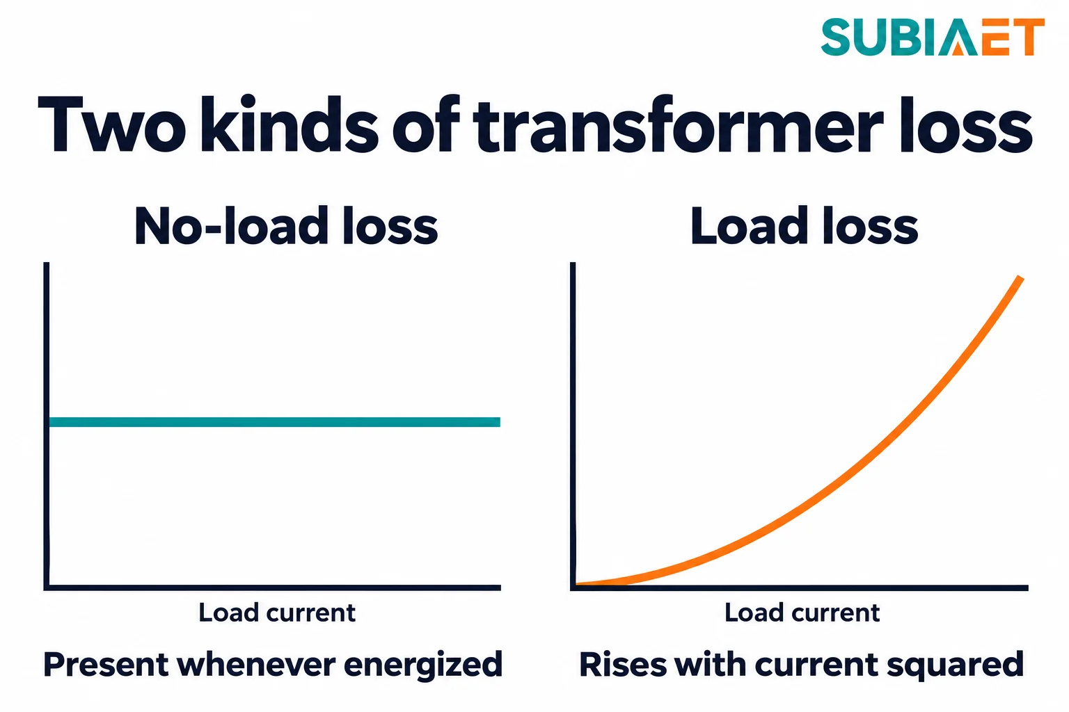
A transformer consumes active power in two different ways, and the two behave in nearly opposite ways as load changes.

No-load loss (P0) is the active power drawn at rated voltage and rated frequency with the other winding open. It comes chiefly from losses in the energized core and persists when connected loads are idle. For this estimate, treat P0 as constant at the assumed voltage and frequency. It contributes during all energized hours, whether the unit is carrying little current or its full operating load.

Load loss (Pk) is the active power at rated current (or at a stated tapping current) and rated frequency, for a stated winding pair and a stated reference temperature. It includes resistive winding losses and additional load-related losses, including winding eddy-current and other stray losses. Unlike no-load loss, it scales with current: at any load current, the load loss is approximately

P_load ≈ Pk × k², where k = RMS load current ÷ corresponding rated or tapping current on the same winding.

At half of rated current, load loss is about a quarter of Pk, not half. At 25% current it is about one-sixteenth. This square law is the single most important thing to internalize before reading a quotation, because it means no-load loss can form a large share of loss energy when a unit spends many energized hours at light load. The actual share still depends on its P0 and Pk.

These are the loss terms as defined in the IEC 60076-1 vocabulary (§3.6 of the 2011 edition, as reproduced in the publicly accessible GSO adoption preview of that edition; the preview is a historical adoption document, cited here for terminology rather than as evidence of any product’s conformity). Three details in that vocabulary matter for quoting: the definitions use the principal tapping unless another tapping is stated, load loss belongs to a specific winding pair, and auxiliary plant consumption is stated separately from the two main loss figures.

How to Calculate Annual Transformer Loss Energy in kWh

A quotation states losses in kilowatts. The energy portion of an electricity bill uses kilowatt-hours; other tariff charges are considered separately. Converting one to the other requires the operating hours, and the conversion differs for the two components:

E ≈ P0 × H_energized + Pk × Σ(hours_i × k_i²)

where the intervals i partition the energized hours, so Σ hours_i = H_energized. De-energized periods contribute neither term: no energized no-load loss and no load-current loss during those intervals.

The UNEP United for Efficiency load-profile method uses squared-current duration weighting. Three qualifications determine whether the estimate suits a project.

• Do not square the average current. If a transformer runs 4,000 hours a year at no load and 4,000 hours at rated current, Σ(h × k²) = 4,000 × 1² = 4,000. Squaring the average fraction (0.5² × 8,000) gives 2,000 — half the correct squared-current duration term, because the loss curve is convex and averaging must be done on the squared quantity, not the raw one.
• Voltage, waveform and balance. P0 is quoted at stated voltage and frequency; changes in those conditions can change no-load loss. The k² estimate assumes roughly balanced, sinusoidal duty. Total RMS current alone does not represent all frequency-dependent losses under substantial harmonic distortion, and phase imbalance also needs appropriate treatment. Those cases require a supplier or engineering model for the actual duty.
• Reference temperature. Winding resistance rises with temperature, so Pk quoted at one reference temperature is a different number from Pk quoted at another. The two bids must be normalized to the same reference before either is used.

Where the unit has fans, pumps or other auxiliaries, account for their energy separately. Use the input power and run time for each relevant operating mode rather than assuming that every accessory runs continuously or draws the same power whenever energized.

The rated current that sets k is not a free number either. For a two-winding unit it follows from rated kVA and rated winding voltage, which is why kVA, kW and power factor have to be read together; comparing a load fraction computed on the LV side against a rated current taken on the HV side produces a meaningless k.

Comparing Two Transformer Quotes Under Light and Heavy Loads

The offer data below is illustrative — two hypothetical offers for an identical two-winding duty, not a market price or any supplier’s quotation. The point is the method, and the numbers are chosen so the arithmetic can be checked by hand.

Offer A is the cheaper unit with the higher standing loss; offer B costs more and has roughly half the no-load loss, but 1 kW more load loss at rated current. Which is “better” is not a property of the transformers — it is a property of the duty.

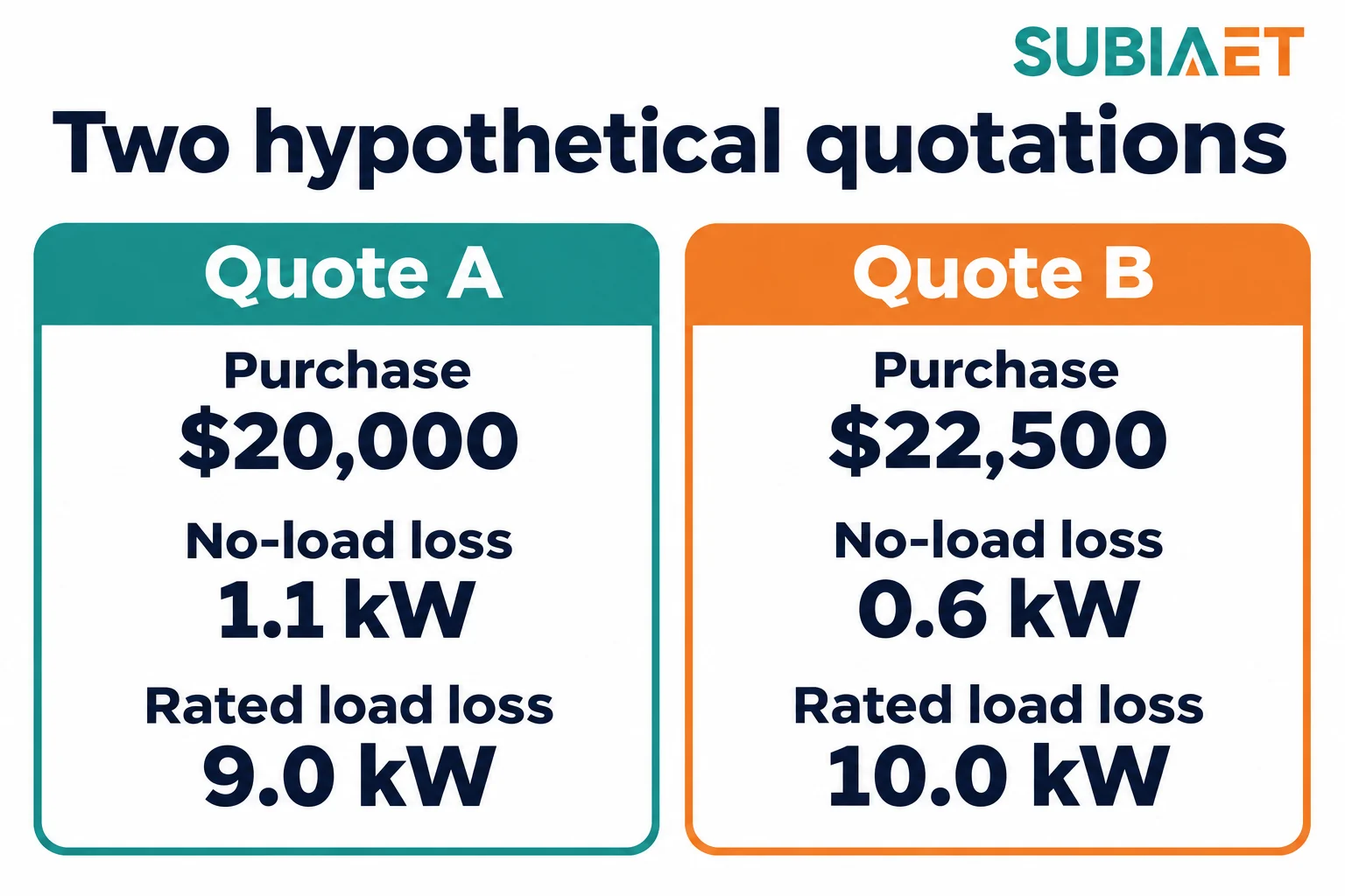
Both profiles assume 8,000 energized hours per year, with the remaining 760 hours de-energized. They differ only in the mix of current levels during those hours.

• Light profile: 6,000 hours at 25% current plus 2,000 hours at 50%. The squared fractions are 0.0625 and 0.25. Their contributions are 6,000 × 0.0625 = 375 hours and 2,000 × 0.25 = 500 hours, giving 875 equivalent full-current hours.
• Heavy profile: 2,000 hours at 50% current plus 6,000 hours at 100%. Their contributions are 2,000 × 0.25 = 500 hours and 6,000 × 1.00 = 6,000 hours, giving 6,500 equivalent full-current hours.

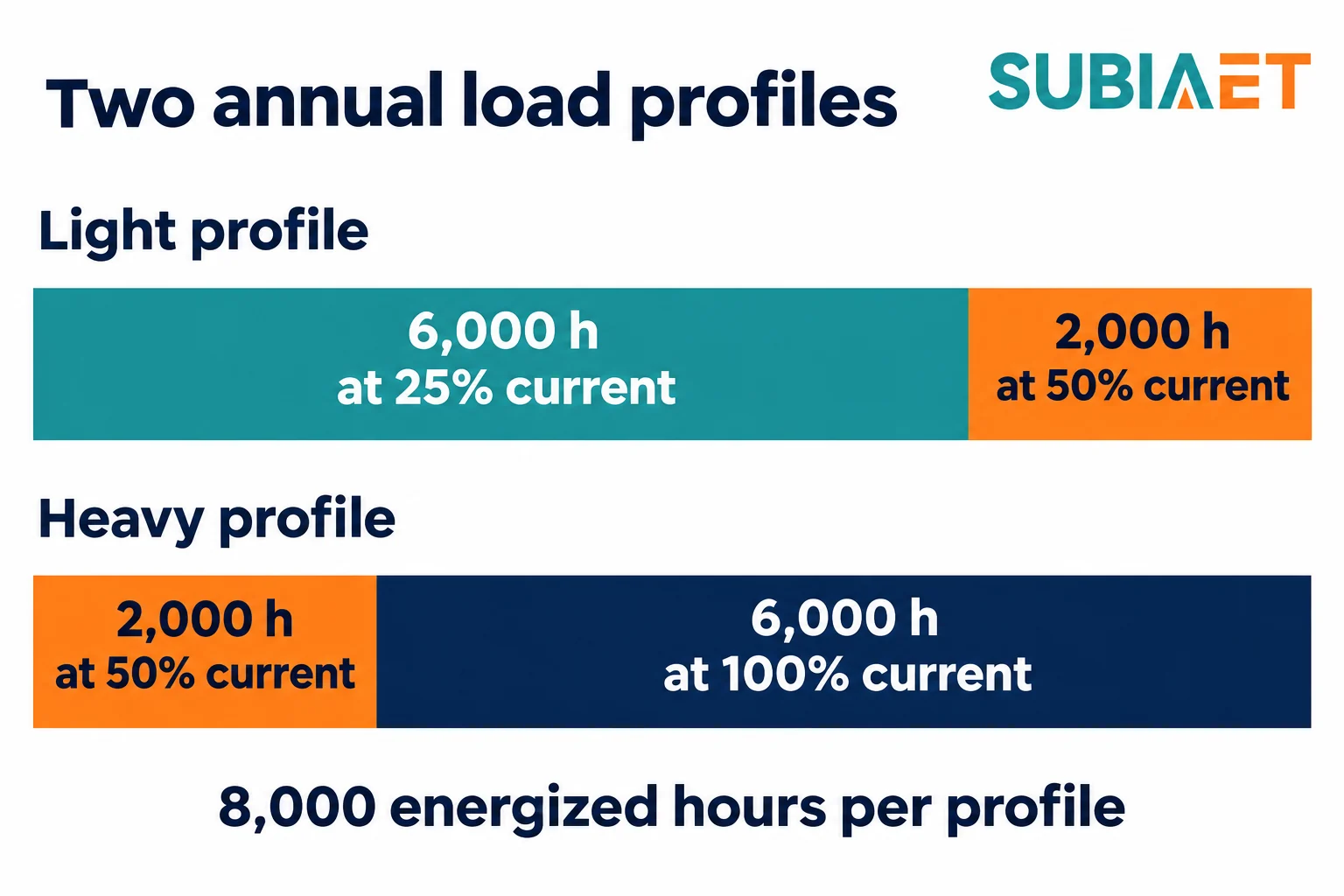
The two duty totals differ by a factor of about 7.4 — 875 equivalent hours against 6,500 — even though both transformers are energized for exactly the same 8,000 hours. That difference changes the operating-cost comparison, which must then be considered with the purchase-price difference.

One complete calculation

Offer A, light profile:

• No-load energy: 1.1 kW × 8,000 h = 8,800 kWh
• Load energy: 9.0 kW × (6,000 h × 0.25² + 2,000 h × 0.50²)
  = 9.0 kW × (375 h + 500 h)
  = 9.0 kW × 875 h = 7,875 kWh
• Annual total: 8,800 + 7,875 = 16,675 kWh

The same procedure for the other three combinations gives:

Under light duty, B’s lower standing loss cuts annual energy by 3,125 kWh despite its higher Pk. Under heavy duty the square law works the other way: B’s extra 1 kW of Pk produces 6,000 kWh of additional energy during the full-current interval plus 500 kWh during the half-current interval. That 6,500 kWh total more than offsets its 4,000 kWh no-load advantage.

How to Calculate the Present Value of Transformer Losses

With the positive discount rate assumed here, energy-cost savings in year 9 have a lower present value than the same money saved today. The assumption set used here: a constant real energy price of $0.12/kWh, a 12-year evaluation horizon, a 5% real annual discount rate, unchanged duty over the horizon, purchase paid now, and energy costs incurred at the end of each year. Pairing a constant real price with a real discount rate keeps inflation out of both sides of the calculation, and constant duty with end-of-year payments collapses the 12 annual energy costs into a single annuity factor:

(1 − 1.05⁻¹²) ÷ 0.05 = 8.86325

The UNEP procurement guide explains the wider loss-capitalization method.

At $0.12/kWh the ranking reverses between the two duties. On light duty B is lower by about $824; on heavy duty A is lower by about $5,159. Differences are computed from unrounded values and then rounded, so the last digit may not tie exactly to the displayed columns.

Why the premium pays back under light duty and not under heavy duty

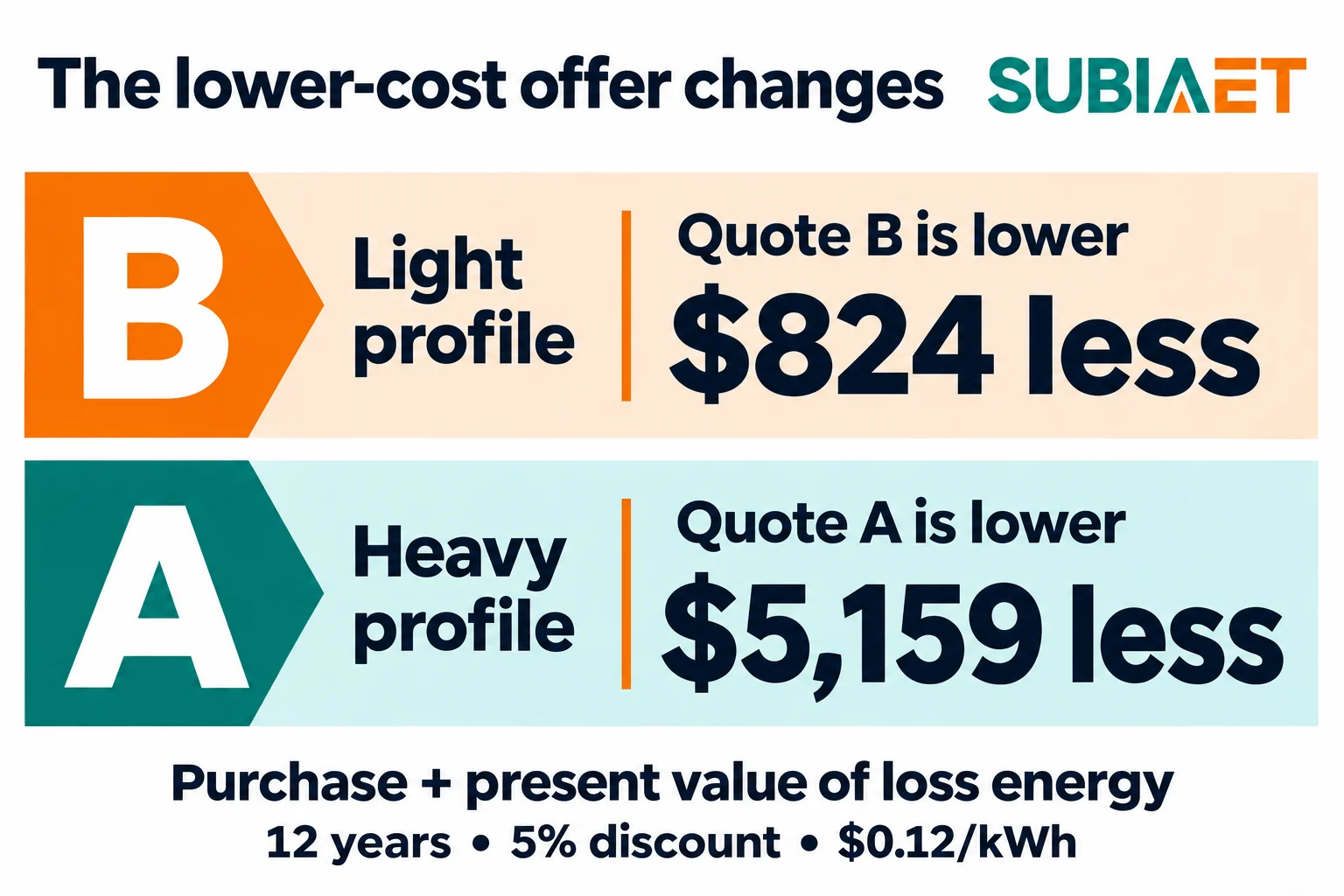
The mechanism is easier to see as a discounted savings test. B’s extra $2,500 at purchase has to be recovered from cheaper operation, and at a 5% real rate over 12 years each $1 per year of saving is worth $8.86 today. Dividing, B needs to save about $282 per year in energy to justify its premium.

• Under light duty, B saves $2,001 − $1,626 = $375 per year — above the threshold, so B wins, and the margin is (375 × 8.86325) − 2,500 ≈ $824.
• Under heavy duty, B does not save at all; it costs $8,376 − $8,076 = $300 per year more, which is (300 × 8.86325) + 2,500 ≈ $5,159 against it.

The direction of the discounting matters for how hard the premium has to work. A longer horizon or a lower discount rate raises the annuity factor and makes future loss savings worth more today, which favours an offer with lower annual loss energy under the selected duty; a shorter horizon or a higher cost of capital does the opposite. The break-even point is therefore a statement about the buyer’s assumptions as much as about the equipment.

Break-Even Electricity Price and Cost Sensitivity

Holding everything else constant and dropping the energy price to $0.08/kWh:

A now leads by about $284 — the reversal simply moved. B’s $375/yr saving at $0.12/kWh becomes $250/yr at $0.08/kWh, which is below the $282/yr threshold its premium requires, so the cheaper unit regains the lead.

Solving for the price at which the light-duty totals are equal gives approximately $0.0903/kWh: the $2,500 premium divided by 3,125 kWh per year multiplied by the 12-year present-value factor of 8.86325. That figure is a sensitivity result for these two hypothetical offers under these assumptions, not a tariff, a market threshold or a recommendation. Above it under light duty, B is cheaper; below it, A is.

What Transformer Total Cost of Ownership Includes

The totals above include purchase and loss energy only. Depending on the project, several other items can be material enough to move the ranking and should be added explicitly rather than absorbed into a vague allowance:

• auxiliary power for fans, pumps and controls, on its own hours-of-operation basis;
• delivery, installation, commissioning, foundations, cable terminations and any civil work;
• maintenance and inspection over the horizon, including any oil testing regime for liquid-immersed units;
• demand or capacity charges where the local tariff structure applies them, recorded once and not double-counted against the energy term;
• end-of-horizon disposal cost and residual value, without counting the same scrap or residual value twice.

A utility valuing losses with its own capital and energy assumptions and a factory valuing them against a purchased tariff are doing different arithmetic on the same kilowatts; the two loss valuations should not be mixed within one comparison. The Bonneville Power Administration assessment discusses loading, energy prices and financing in utility loss valuations.

How to Compare Transformer Loss Guarantees Across Quotes

None of the arithmetic above means anything if the two quotations describe different things. The sequence is: confirm both offers meet the electrical and installation duty, then normalize the loss figures, then evaluate.

Confirm the duty first. Both units must meet the same required electrical and installation duty: kVA under the stated conditions, voltage ratio, frequency, relevant impedance and tap requirements, cooling performance, temperature-rise limits and installation environment. They need not have identical construction or every numerical parameter, but departures from the specification must be evaluated before using the cost ranking. A different cooling stage or tap assumption should be visible as a qualification.

Then put the losses on one basis. For each offer, record:

• P0 and Pk separately, in kW, not a combined “total loss” or an efficiency percentage at an unspecified load;
• the rated kVA, voltage and frequency at which those figures apply;
• the tapping — principal tapping unless the offer states otherwise;
• the winding pair the load loss refers to;
• the reference temperature for load loss;
• whether each figure is a guaranteed value or a typical/calculated value, and on what tolerance basis;
• what the stated auxiliary power covers, at which operating condition, and where in the document it appears.

A guaranteed figure carrying a tolerance band and a “typical” figure from a calculation sheet are not the same kind of claim, and treating them as interchangeable can manufacture a difference that does not exist or hide one that does. Where a bidder supplies only efficiency at 50% load, ask for P0 and Pk at the same reference conditions as the other offer rather than reversing the formula by rule of thumb.

Two supporting steps are worth doing before the evaluation itself. Getting the load data right is the same exercise as any factory expansion sizing study, where interval-by-interval demand records replace assumed bins. And the industrial transformer selection and quotation workflow covers the ordering of duty definition, technical comparison and commercial comparison that this evaluation assumes.

Next steps for a live comparison

If you are holding two real quotations now, the practical sequence is:

1. Fix the operating profile from interval meter data or a defensible load estimate, in bins that sum to the energized hours, and state whether the unit is switched off during shutdown periods.
2. Normalize both offers to the same kVA, tapping, winding pair and load-loss reference temperature, and separate guaranteed from typical values.
3. Apply your own energy price, horizon and discount rate — not the ones in this article — and compute evaluated totals for each profile you might actually operate.
4. Run one sensitivity at a lower and a higher energy price to see how close the ranking sits to its break-even point.
5. Add the non-loss cost items that are material for your site before signing, so the comparison reflects the stated ownership-cost scope rather than purchase price alone.

The transformer product families cover liquid-immersed, dry-type, pad-mounted and power transformer configurations; which family suits a given installation is a separate decision driven by the environment, and the oil-immersed versus dry-type selection comparison sets out those conditions. The energy-accounting method can be applied to either family when its assumptions fit. Use the actual loss reference conditions, loading and auxiliary energy for each candidate rather than assuming P0 and Pk are the only differences.

FAQ

Does a transformer still consume energy when it is idle?

Yes. An energized transformer draws no-load power even when the connected equipment is idle. Multiply its estimated no-load kW by its energized hours to estimate that part of the loss energy.

Why use current squared for each interval?

Load loss rises approximately with the square of current under the stated assumptions. Squaring each interval first gives high-current hours their correct weight. Squaring the average first understates the estimate when current varies.

Can a transformer with a lower no-load loss cost more to run?

Yes. Higher load loss can outweigh lower no-load loss if the unit spends enough time near rated current. Evaluate both losses against the same load profile.

What if the quotes use different loss-test conditions?

Ask for separate no-load and load-loss figures on the agreed basis. Match the relevant voltage and frequency, tap, winding pair, current and load-loss reference temperature. Confirm which figures are guaranteed and whether auxiliaries are quoted separately.